How plumber Turns Your R Scripts into On-Demand Data Faucets

Author

Numbers around us

Published

May 6, 2025

💧 Introduction

Imagine if your data could flow like water — available when needed, filtered to your taste, and ready to serve. As R users, we often write powerful analyses that live inside scripts or notebooks, waiting to be rerun or reknit. But what if someone else — a dashboard, a spreadsheet, even a non-technical colleague — could turn a faucet and get just the data or insight they need, right when they need it?

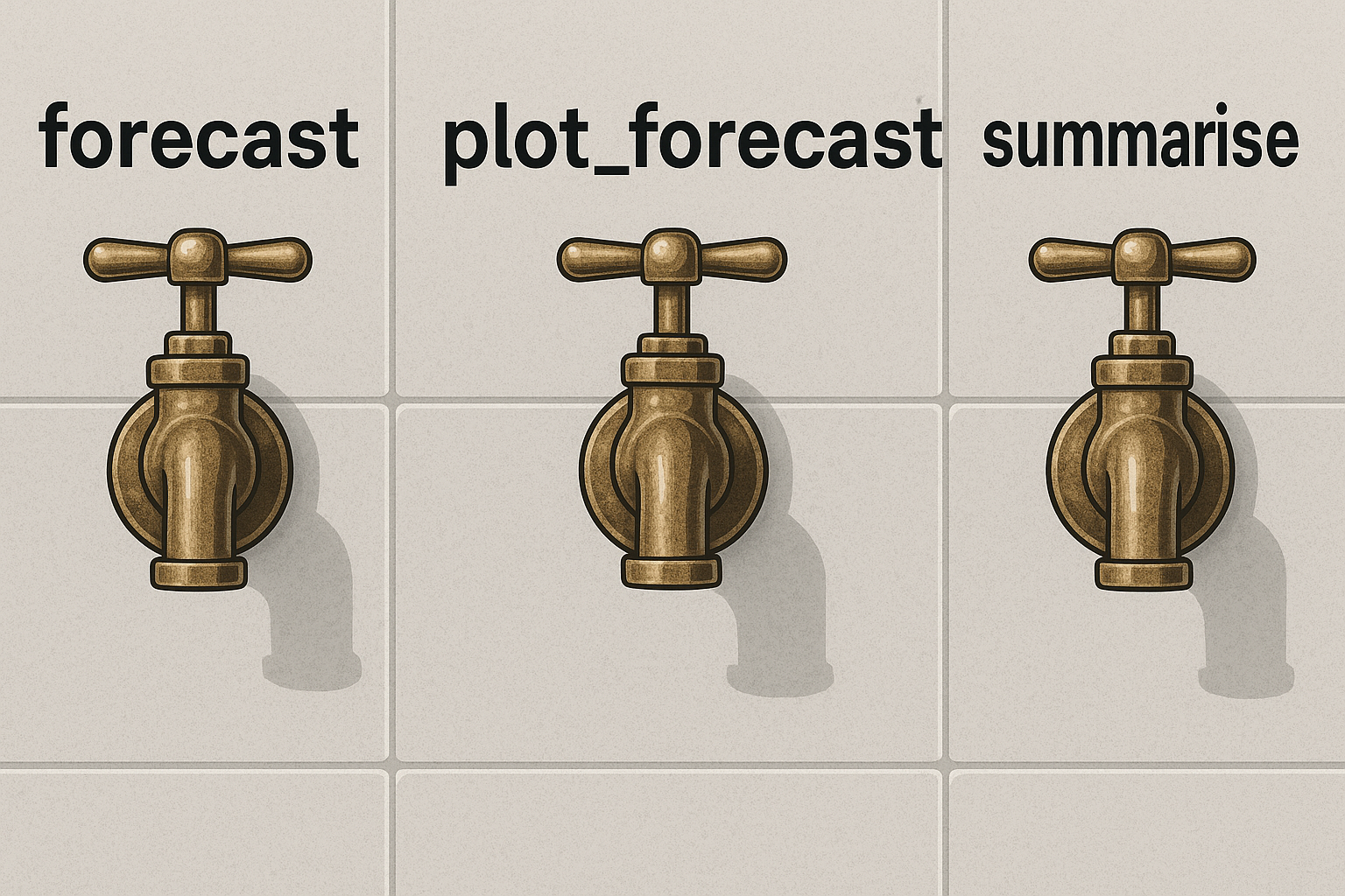
Enter plumber: the package that transforms your R code into web-accessible endpoints. With just a few annotations, you can create lightweight, on-demand services — faucets — that deliver filtered data, summaries, forecasts, and even dynamic plots.

In this tutorial, we’ll build a trio of “data faucets” using the classic gapminder dataset. Each one will be activated via a simple HTTP GET request, controlled through query parameters — just like adjusting the knobs on a sink. No dashboards, no shiny, no server frameworks. Just clean, functional API plumbing in R.

🔧 What is plumber (and what is a data faucet)?

plumber is an R package that exposes R functions as web API endpoints. That means you can call your R code over HTTP — from a browser, a spreadsheet, or another app — and get results back as JSON.

In this metaphor, we’ll treat your code like a faucet. A faucet doesn’t boil water or change its chemistry — it just controls when, where, and how water flows. Similarly, a plumber endpoint gives users access to a very specific piece of logic you’ve defined in R: filter this data, summarize that column, draw a plot. They don’t need to understand the pipework underneath — just turn the handle.

A typical plumber endpoint looks like this:

Code

#* @get /hello
function(name = "World") {
  list(message = paste("Hello,", name))
}

Visiting http://localhost:8000/hello?name=Alice would return:

{
  "message": "Hello, Alice"
}

In the rest of this article, we’ll build more sophisticated faucets — not to say hello, but to summarize, forecast, and visualize data from gapminder.

🌍 Our dataset — a classic reservoir

Before you can open the tap, you need a water supply. In our case, that’s the gapminder dataset — a tidy, time-series snapshot of global development indicators. It’s compact, well-structured, and ideal for building API examples without external dependencies.

Let’s load the dataset and take a quick look:

Code

library(gapminder)
library(dplyr)

data <- gapminder::gapminder
glimpse(data)

You’ll see six columns:

country: Name of the country
continent: Continent the country belongs to
year: Observation year (1952–2007 in 5-year steps)
lifeExp: Life expectancy
pop: Population
gdpPercap: GDP per capita

Think of this dataset as a water tank — structured, pressurized, and ready to be tapped. Every API call we’ll build will draw from this tank, apply some filtering or transformation, and return a clean stream of results.

Here’s a simple example using dplyr to filter the data manually — we’ll soon automate this behind an endpoint:

Code

data %>%
  filter(country == "Poland", year >= 1972, year <= 2002) %>%
  select(year, lifeExp)

This snippet answers a narrow question: How has life expectancy changed in Poland between 1972 and 2002?

Now let’s build a faucet that does this — on demand.

Faucet 1 — Data summary on request

Our first faucet delivers summary statistics for any country and development metric in the dataset. Think of it as a cold-water tap: you specify the country and the metric, and it returns a quick, refreshing snapshot — no modeling, no visualization, just facts.

💡 Example request:

GET /summary?country=Poland&metric=lifeExp

Expected response:

{
  "country": "Poland",
  "metric": "lifeExp",
  "min": 61.0,
  "max": 75.5,
  "mean": 70.34,
  "median": 71.0,
  "latest": 75.5
}

🧠 Behind the faucet: the R function

Let’s write an R function that accepts a country and a metric, filters the dataset accordingly, and returns a named list of basic statistics:

Code

summary_stats <- function(data, country, metric) {
  if (!(metric %in% names(data))) {
    stop("Metric not found in dataset")
  }

  df <- data %>% 
    filter(country == !!country) %>%
    select(year, value = all_of(metric)) %>%
    arrange(year)

  if (nrow(df) == 0) {
    stop("No data found for selected country")
  }

  list(
    country = country,
    metric = metric,
    min = min(df$value, na.rm = TRUE),
    max = max(df$value, na.rm = TRUE),
    mean = mean(df$value, na.rm = TRUE),
    median = median(df$value, na.rm = TRUE),
    latest = tail(df$value, 1)
  )
}

🔌 Exposing the faucet with plumber

Now we add this function to a plumber route. Here’s how to define a /summary endpoint that accepts query parameters for country and metric:

Code

# plumber.R
#* @param country The name of the country (e.g. "Poland")
#* @param metric The metric to summarize (e.g. "lifeExp", "gdpPercap")
#* @get /summary
function(country = "", metric = "lifeExp") {
  tryCatch({
    summary_stats(data, country, metric)
  }, error = function(e) {
    list(error = e$message)
  })
}

Save this file and launch the API with:

Code

pr <- plumber::plumb("plumber.R")
pr$run(port = 8000)

Now try visiting:

http://localhost:8000/summary?country=Poland&metric=lifeExp

💡 Tip: if you get an error, check spelling — plumber doesn’t do autocomplete!

You’ve now built your first live data faucet: users can request a country and a metric, and get real-time stats — no dashboards, no spreadsheets.

🔥 Faucet 2 — Forecasting future flow

Our next faucet doesn’t just report the past — it predicts the future. Given a country, a metric (like life expectancy), and a time range, it builds a linear trend model and forecasts future values for a specified horizon.

Think of this as a hot water tap: it uses energy (a model) to project where things are going — not just where they’ve been.

💡 Example request:

GET /forecast?country=Poland&metric=lifeExp&from=1972&to=2002&horizon=10

Expected response (truncated):

[
  { "year": 1972, "value": 70.1 },
  ...
  { "year": 2002, "value": 75.5 },
  { "year": 2007, "value": 76.4 },
  { "year": 2012, "value": 77.3 }
]

🔧 Modeling the future with `lm()`

Let’s write a function that:

Filters the dataset by country and year range
Fits a linear regression model (lm(value ~ year))
Forecasts horizon years into the future (at 5-year intervals)

Code

forecast_lm <- function(data, country, metric, from, to, horizon = 10) {
  df <- data %>%
    filter(country == !!country, year >= from, year <= to) %>%
    select(year, value = all_of(metric)) %>%
    arrange(year)

  if (nrow(df) < 3) stop("Not enough data points to build a model")

  model <- lm(value ~ year, data = df)

  last_year <- max(df$year)
  future_years <- tibble(year = seq(last_year + 5, last_year + horizon, by = 5))
  preds <- predict(model, newdata = future_years)

  forecast <- bind_rows(
    df,
    tibble(year = future_years$year, value = preds)
  )

  forecast
}

🧩 Creating the /forecast endpoint

Code

# plumber.R
#* @param country Country name
#* @param metric Metric to forecast
#* @param from Start year
#* @param to End year
#* @param horizon Years to forecast beyond `to`
#* @get /forecast
function(country = "", metric = "lifeExp", from = 1962, to = 2007, horizon = 10) {
  tryCatch({
    from <- as.numeric(from)
    to <- as.numeric(to)
    horizon <- as.numeric(horizon)

    result <- forecast_lm(data, country, metric, from, to, horizon)
    result
  }, error = function(e) {
    list(error = e$message)
  })
}

Start or reload your plumber API, then try:

http://localhost:8000/forecast?country=Poland&metric=lifeExp&from=1972&to=2002&horizon=10

You now have a faucet that models and delivers future insights on the fly.

🖼️ Faucet 3 — Line chart with a twist

So far, your API can serve stats and forecasts — but sometimes numbers just don’t flow as well as pictures. This final faucet will return a line chart showing the historical and forecasted values as a single visual stream.

This is the designer faucet — it doesn’t just give you water, it does it with flair.

💡 Example request:

GET /forecast?country=Poland&metric=lifeExp&from=1972&to=2002&horizon=10&plot=true

Expected response:

{
  "plot": "data:image/png;base64,iVBORw0KGgoAAAANSUhEUgAA..."
}

This base64-encoded string can be rendered directly in an HTML img tag, embedded in dashboards, or downloaded as a PNG.

🖌 Generating the plot

We’ll use ggplot2 to draw the chart and base64enc to encode the image for API delivery.

Code

library(ggplot2)
library(base64enc)

plot_forecast <- function(df, country, metric) {
  p <- ggplot(df, aes(x = year, y = value)) +
    geom_line(color = "steelblue", size = 1) +
    geom_point(size = 2) +
    theme_minimal() +
    labs(
      title = paste("Forecast for", country),
      y = metric, x = "Year"
    )

  tf <- tempfile(fileext = ".png")
  ggsave(tf, plot = p, width = 6, height = 4, dpi = 150)
  dataURI(file = tf, mime = "image/png")
}

🧩 Updating the `/forecast` endpoint with `plot=TRUE`

Let’s update the existing endpoint to return either raw data or a plot, based on a plot parameter:

Code

#* @serializer contentType list(type='image/png')
#* @get /forecast
function(country = "", metric = "lifeExp", from = 1962, to = 2007, horizon = 10, plot = "false") {
  tryCatch({
    from <- as.numeric(from)
    to <- as.numeric(to)
    horizon <- as.numeric(horizon)
    plot <- tolower(plot) == "true"

    result <- forecast_lm(data, country, metric, from, to, horizon)

    if (plot) {
      p <- ggplot(result, aes(x = year, y = value)) +
        geom_line(color = "steelblue", size = 1) +
        geom_point(size = 2) +
        theme_minimal() +
        labs(
          title = paste("Forecast for", country),
          y = metric, x = "Year"
        )

      tf <- tempfile(fileext = ".png")
      ggsave(tf, plot = p, width = 6, height = 4, dpi = 150)

      # Return file connection (plumber will serve it directly as image/png)
      readBin(tf, "raw", n = file.info(tf)$size)
    } else {
      result
    }
  }, error = function(e) {
    list(error = e$message)
  })
}

🧪 Test the PNG response

Visit this in your browser:

http://localhost:8000/forecast?country=Poland&metric=lifeExp&from=1972&to=2002&horizon=10&plot=true

🛠️ Putting it all together

At this point, you’ve built a small but mighty collection of data faucets:

/summary delivers quick statistics based on country and metric
/forecast returns a time-extended series — either as JSON or as a real PNG chart
You’ve used plumber to wire up these faucets into accessible, browser-friendly endpoints

Now let’s look at how to organize and run this whole system.

🔧 Final `plumber.R` file (minimal, modular version)

Code

library(plumber)
library(dplyr)
library(gapminder)
library(ggplot2)

data <- gapminder::gapminder

# Summary function
summary_stats <- function(data, country, metric) {
  if (!(metric %in% names(data))) stop("Metric not found")
  df <- data %>%
    filter(country == !!country) %>%
    select(year, value = all_of(metric)) %>%
    arrange(year)
  if (nrow(df) == 0) stop("No data found")

  list(
    country = country,
    metric = metric,
    min = min(df$value, na.rm = TRUE),
    max = max(df$value, na.rm = TRUE),
    mean = mean(df$value, na.rm = TRUE),
    median = median(df$value, na.rm = TRUE),
    latest = tail(df$value, 1)
  )
}

# Forecast function
forecast_lm <- function(data, country, metric, from, to, horizon) {
  df <- data %>%
    filter(country == !!country, year >= from, year <= to) %>%
    select(year, value = all_of(metric)) %>%
    arrange(year)
  if (nrow(df) < 3) stop("Not enough data")

  model <- lm(value ~ year, data = df)
  future_years <- tibble(year = seq(max(df$year) + 5, max(df$year) + horizon, by = 5))
  preds <- predict(model, newdata = future_years)

  bind_rows(df, tibble(year = future_years$year, value = preds))
}

#* @get /summary
function(country = "", metric = "lifeExp") {
  tryCatch({
    summary_stats(data, country, metric)
  }, error = function(e) list(error = e$message))
}

#* @serializer contentType list(type='image/png')
#* @get /forecast
function(country = "", metric = "lifeExp", from = 1962, to = 2007, horizon = 10, plot = "false") {
  tryCatch({
    from <- as.numeric(from)
    to <- as.numeric(to)
    horizon <- as.numeric(horizon)
    plot <- tolower(plot) == "true"

    result <- forecast_lm(data, country, metric, from, to, horizon)

    if (plot) {
      p <- ggplot(result, aes(x = year, y = value)) +
        geom_line(color = "steelblue", size = 1) +
        geom_point(size = 2) +
        theme_minimal() +
        labs(title = paste("Forecast for", country), y = metric, x = "Year")

      tf <- tempfile(fileext = ".png")
      ggsave(tf, plot = p, width = 6, height = 4, dpi = 150)
      readBin(tf, "raw", n = file.info(tf)$size)
    } else {
      result
    }
  }, error = function(e) list(error = e$message))
}

▶️ Running the API

In a script or console:

Code

pr <- plumber::plumb("plumber.R")
pr$run(port = 8000)

You now have a live REST API with:

GET /summary?country=Sweden&metric=lifeExp
GET /forecast?country=Poland&from=1972&to=2002&horizon=10
GET /forecast?country=Poland&plot=true → returns image

This can be accessed from:

Web browsers
R, Python, JS clients
Excel or Power BI as a Web data source
Scheduled scripts or cron jobs

🧩 Real-world use cases

Building an API in R isn’t just a neat exercise — it opens doors to automation, collaboration, and smarter data workflows. Here’s how you can put your new set of data faucets to work in the wild.

💼 1. Business dashboards (without Shiny)

Have a team that needs to monitor key indicators — like GDP, life expectancy, or population trends — but doesn’t need interactive Shiny apps?

Serve your forecasts or summaries as JSON to tools like Power BI, Google Sheets, or Grafana.
Point a GET request at your /summary or /forecast endpoint.
Bonus: use query parameters to adjust country, metric, or time range dynamically.

📈 2. Report automation with Quarto

Want a PDF or HTML report that updates automatically every week?

In your Quarto document, call the API using httr::GET() or jsonlite::fromJSON().
Pull in fresh forecasts or visuals just before knitting.
Schedule the report generation via cron, GitHub Actions, or RStudio Connect.

Example code block in R Markdown:

Code

response <- jsonlite::fromJSON("http://localhost:8000/summary?country=Kenya&metric=lifeExp")

🤝 3. Cross-language collaboration

Have Python developers or JavaScript apps that need data from your R analysis?

No need to share scripts or environments — just provide API access.
Python client example:

Code

import requests
response = requests.get("http://localhost:8000/summary", params={"country": "Norway"})
print(response.json())

Works with any language that can make HTTP requests.

📤 4. Batch forecasting or scheduled predictions

Want to auto-refresh 5-year projections for 100 countries?

Write an R script that loops through countries, hits /forecast, and saves the results.
Useful for building datasets, dashboards, or feeding a downstream model.

🌍 5. Public-facing endpoints

If your data is safe to share, expose endpoints externally (e.g. via ShinyApps.io, Posit Connect, or a lightweight cloud server). You’ll have:

Educational tools for students and journalists
Interactive demos for workshops
Lightweight alternatives to heavy web apps

Just be sure to handle request limits, logging, and basic input validation.

Even without a frontend or database, your plumber API becomes a flexible, modular backbone for all kinds of data delivery — internal or external, on-demand or automated.

🧾 Conclusion: small faucets, big flow

You didn’t build a dashboard.
You didn’t deploy a full app.
And yet, with just a few lines of R and plumber, you created something powerful: an accessible, reusable, on-demand interface to your data.

By treating your analysis like plumbing — with controlled flow, modular design, and clean output — you’ve turned raw R scripts into living services. Whether it’s a quick summary, a forward-looking forecast, or a real-time chart, your data is now:

Self-serve
Language-agnostic
Reusable
Ready for production (or a very elegant hack)

And best of all: you’re still just writing R.

🛠 What’s next?

Here are a few ways you can evolve this system:

🧮 Swap in more powerful models: Try prophet, ARIMA, or fable instead of lm()
🌍 Add geo endpoints: Return top countries by growth or metrics per continent
📦 Connect to real data: Read from a live database or API instead of gapminder
🧪 Add tests: Use testthat to validate endpoints and logic
🚀 Deploy it: Host it via Docker, Posit Connect, or a simple VPS with systemd

The key takeaway?
APIs don’t need to be heavy, complex, or coupled to ML.
Sometimes, a clean faucet with exactly the data you want is more than enough.

💧 Introduction

🔧 What is plumber (and what is a data faucet)?

🌍 Our dataset — a classic reservoir

Faucet 1 — Data summary on request

🧠 Behind the faucet: the R function

🔌 Exposing the faucet with plumber

🔥 Faucet 2 — Forecasting future flow

🔧 Modeling the future with lm()

🖼️ Faucet 3 — Line chart with a twist

🖌 Generating the plot

🧩 Updating the /forecast endpoint with plot=TRUE

🧪 Test the PNG response

🛠️ Putting it all together

🔧 Final plumber.R file (minimal, modular version)

▶️ Running the API

🧩 Real-world use cases

💼 1. Business dashboards (without Shiny)

📈 2. Report automation with Quarto

🤝 3. Cross-language collaboration

📤 4. Batch forecasting or scheduled predictions

🌍 5. Public-facing endpoints

🧾 Conclusion: small faucets, big flow

🛠 What’s next?

🔧 Modeling the future with `lm()`

🧩 Updating the `/forecast` endpoint with `plot=TRUE`

🔧 Final `plumber.R` file (minimal, modular version)